SAE report — layer12_topk_k32_dict8x

TopK SAE on Gemma 2 2B layer-12 residual activations, trained on the 500k-token harvest.

Training curves

Reconstruction loss (raw MSE)

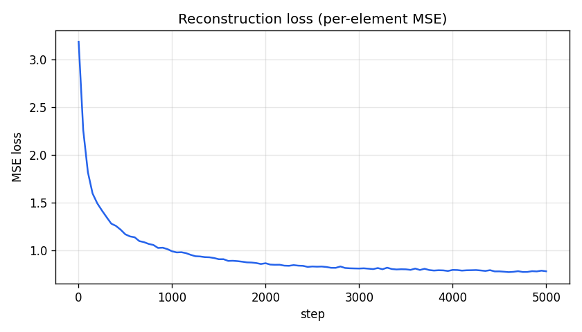
Per-element squared error between input activations and the SAE's reconstruction. Monotone decrease confirms the optimizer is making progress. Note the y-axis is the average squared error per residual dimension — the absolute number depends on the activation scale (Gemma-2-2b layer 12 has fp16 activations with O(10) per-dim magnitude).

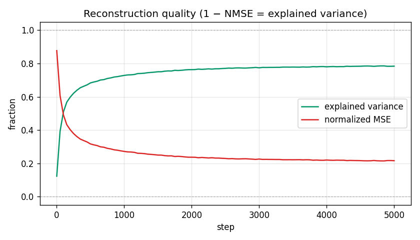
Explained variance & normalized MSE

This is the “accuracy” metric for SAEs. There is no classification accuracy because the task is reconstruction. Normalized MSE divides each example's squared error by its squared distance from the dataset mean, so a trivial mean-predictor gets NMSE = 1.0 (EV = 0); perfect recon gets NMSE = 0 (EV = 1). Our run ends at EV ≈ 0.78 — the SAE captures ~78% of the residual-stream variance using only k = 32 features per token.

L0 sparsity

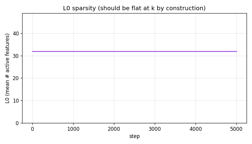
Average number of nonzero features per token. With TopK this is exactly k by construction — useful only as a sanity check that the TopK op is wired correctly. With L1-penalized SAEs this curve drifts and tuning it is the whole game.

Dead-feature fraction

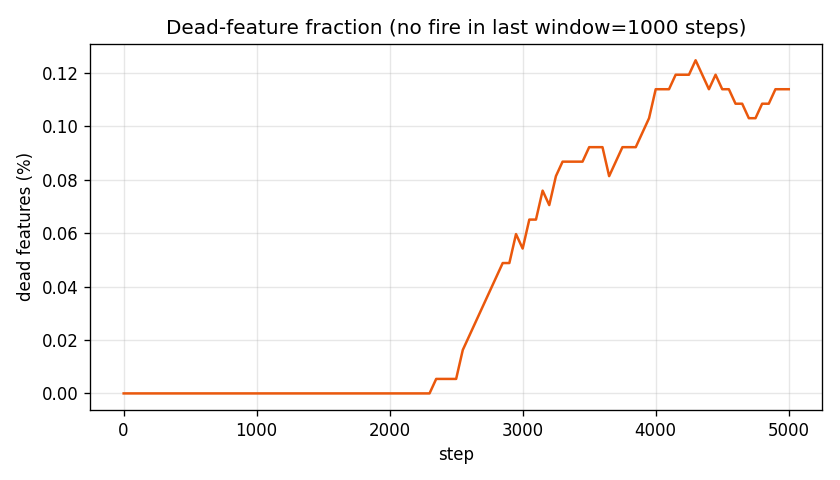
Fraction of features whose pre-activation has not entered any token's top-k for the past 1000 steps. Once a feature stops firing it stops getting gradient and tends to stay dead. Our run plateaus at ~21 dead features (0.11%) — small enough that resampling isn't worth implementing yet. For larger dictionaries (32× and up) this is the headline failure mode.

Per-batch feature usage

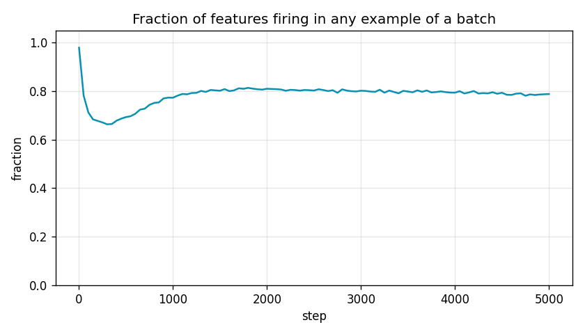
Fraction of features that fire in at least one example of the current batch. At init nearly all features fire on random inputs (~98%). The dip around step 100–500 is the encoder specializing. The rebound to ~80% is the model rediscovering the broad set; the gap from 100% is partly batch noise and partly genuinely-rare features.

Post-hoc feature diagnostics

Computed by loading the final checkpoint and forward-passing a fresh sample of 50,000 tokens.

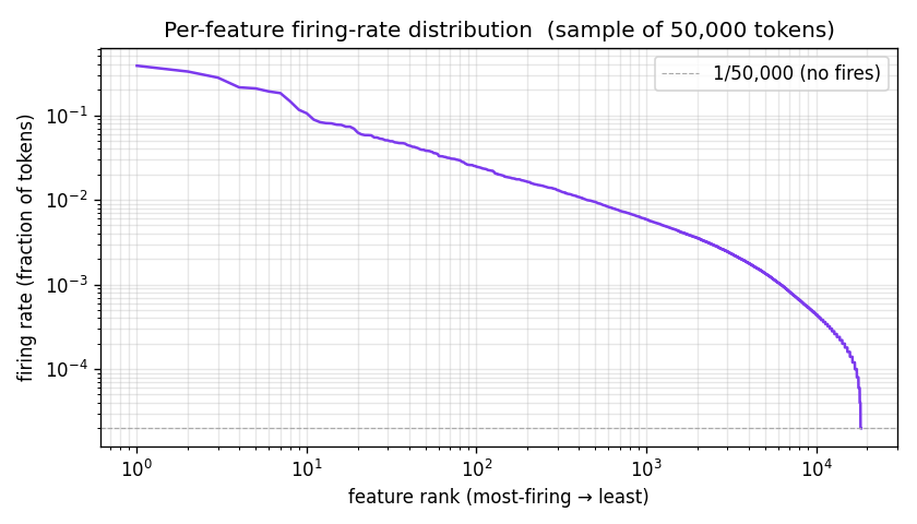
Per-feature firing-rate distribution (log-log)

Sort all 18,432 features by how often they fired across the sample, then plot rank vs firing-rate on log-log axes. A healthy SAE shows a roughly power-law distribution: a few very-frequent features (function words, common contexts) and a long tail of rare-but-specific features. Hard floor at 1/n_sample marks "never fired in this sample" — the count after the cliff is the empirical dead count.

Decoder row norms

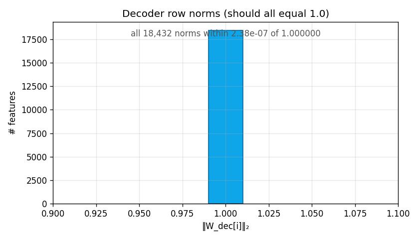
Sanity check: normalize_decoder() should keep every row of W_dec at exactly unit norm. The histogram should be a single spike at 1.0. Any spread means the projection step is broken.

What we did not measure (yet)

Standard SAE diagnostics in the literature that aren't in this report:

Substitution loss / CE-delta — the gold standard. Run Gemma on real text, replace layer-12's residual stream with the SAE's reconstruction, and measure how much the downstream cross-entropy loss increases. A perfect SAE leaves CE unchanged. Anthropic's papers quote this as the headline number. We need the model loaded to compute it; cheap to add as a separate eval script.
Per-feature reconstruction contribution — for each feature i, what fraction of the total recon does it account for? Helps distinguish "high firing rate but low contribution" features (noisy) from "low firing rate but high magnitude" features (specific).
Feature activation magnitude histogram — the distribution of z values when a feature is active. Bimodal/long-tailed magnitudes are healthy; very tight clusters can indicate dead-on-arrival features.
Feature decoder-direction similarity — cosine similarity matrix of W_dec rows. Near-duplicates suggest the dictionary is over-parameterized for the data; orthogonal rows suggest the SAE has found a genuine basis.
Auto-interp (Phase 4 in PLAN.md) — for each feature, collect its top-k max-activating prompts and ask a stronger LM to label what they have in common. The single most useful tool for "did we learn anything?".
Steering — add a decoder direction to the residual stream at inference and observe behavior change. Validates that the feature is causal, not just correlational.
Comparison against Gemma Scope — DeepMind's pretrained SAEs for every Gemma 2 layer. Cosine-match our learned decoder rows against theirs to see which features we found and which we missed.

Ordering by ROI for our project: auto-interp on a handful of features (cheap, tells us if anything is interpretable) → CE-delta eval (cheap, tells us reconstruction is faithful where it matters) → re-harvest more tokens and rerun.

steps	5,000
wall time	4379 s (73.0 min)
final MSE loss	0.7817
final normalized MSE	0.216
final explained variance	78.4%
L0 (target = k)	32.0 (k = 32)
dead features (window=1000)	20 / 18,432 (0.114%)
dead features (sample, no fires in 50k tokens)	67 / 18,432

run name	layer12_topk_k32_dict8x_smoke
source model	google/gemma-2-2b
layer	12
d_model	2304
n_features	18,432 (= 8 × d_model)
k (TopK)	32
batch size	4096
learning rate	0.0003
training steps	5000
seed	0

SAE training report — layer12_topk_k32_dict8x_smoke

Summary